Minesweeper pt. 3: more gameplay

See part 1 for a description of Tile Domination and Gradient.

Adding the feature from part 2, that guarantees that the instances are solvable makes the game much more satisfying. With this knowledge, I could spend all the time thinking of clever inferences, instead of wondering whether the instance is solvable at all. This post contains some interesting cases that I ran into.

Tile Domination

Typical tile domination. The 2 dominates the upper 1 (sees all tiles of it, plus some more)

Tile domination with very good payoff! The yellow tiles contain exactly one mine.

A nice interdependence between the top three middle tiles, give us that the red tile is a mine. Could also be solved with tile domination between the "1" and one of the "2"s.

Gradient

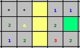
A hard to spot application of the gradient rule. The yellow tiles must contain exactly one mine.

Another hard to spot gradient, between the middle "1" and the middle "3". The yellow tiles contain exactly one mine. 

Global constraint

(counting total number of mines)

Typical application of the global constraint. The colored area is the only unknown area left in the game. The yellow, orange, and turquoise tiles contain exactly one mine each. Since there are only three mines left in the game, the green tiles must be free.

A larger application of the global constraint. The yellow and orange tiles must contain exactly two mines each. The turquoise tiles contain exactly one mine. Therefore, the green tiles are free.

Applying the global constraint with two remaining separate areas. There is just one way to assign two mines so as to "touch" all unsatisfied tiles. 

 Multi-step inferences

Shared tile domination: the "2" on the lower left must be satisfied by the combined yellow and orange tiles.

Proving that the "box" is filled diagonally. I have marked colored boxes around the tiles that yield the conclusions about the colored tiles. The order of reasoning goes first: yellow, orange, purple, and turquoise must all contain one mine, by straight application of adjacency constraints. Then brown is inferred to contain one mine based on orange, purple, and turquoise. With this, we see that the green tiles are free. 

Yellow, turquoise, and brown fields contain one mine by adjacency constraints. From yellow, we get the orange by tile domination. Using the same reasoning about the box as above, the purple must contain one mine, so the green tiles are free by saturation of the right "1". Using the box in the other direction, the tile directly above the left "3" must be free. 

Minesweeper pt. 2: SAT (the cheating button)

Previous:

• Minesweeper Turbo

In the previous post, I applied some more or less simple rules for playing Minesweeper. At the end of it, two issues were raised. First, we would like to generate only problems that we know are solvable. Second, we would like to check whether a certain situation is truly "impossible", or whether we can make more inferences. Both of these features would be simple if we could automatically exhaust all possible inferences for a certain board. This is what SAT will do for us. 

Implementation

The method of determining whether or not tiles are mines will be proof by contradiction. We will set up a SAT model that holds the adjacency constraints. A tile X can be shown to be a mine by showing that "X is free" leads to the SAT model being unsatisfiable. Likewise, X can be shown to be free by showing that "X is mine" makes the SAT model unsatisfiable. 

Aside from the adjacency constraints, we can also add a global constraint on the total number of mines, since this is known to the player. 

For performance reasons, the only unknown tiles considered will be those that touch an open tile. None other are relevant for the adjacency constraints. 

Consequences

Given a method to exhaust all inferences, we can generate solvable instances by running the apply_SAT function to the initial state, and see if it leads to a finished game. If not, generate a new problem and try again. When we are working with a solvable game, we always know that there is at least one way to proceed, at least one tile that can be inferred to be free or a mine. 

For games that are not guaranteed to be solvable, I installed a "cheating button". We can also call it an "answer sheet button". The cheating button runs apply_SAT. If no more tiles open, the situation was actually hopeless.  If some tiles opened, there was something to do. After apply_SAT finishes, however, there is nothing to do. One must simply take a guess. Of course, in Minesweeper we do not care to guess, so mathematically, the game is over. 

Performance

Proving that a given Expert game (16x30 tiles, 99 mines) is unsolvable takes 0.1-1 seconds. Proving that it is solvable is about the same. For a Super-Expert game (30x50 tiles, 300 mines), the time is about 1-10 seconds for proving solvability/unsolvability. Expert games and Super-Expert games are solvable with a rate of about 1 in 10. 

Minesweeper Turbo

Remember minesweeper? You left click to open a tile, and right click to flag it as a mine. When a tile is opened, it displays the number of mines in the 8-connected adjacent tiles. Open a mine and you're dead. You win the game by opening all non-mines.

A finished beginner game: 8x8 tiles, 10 mines.

I started playing it again recently, not having played it for about 10 years. It was fun to attack the game again with a more "adult" brain. More patience and experience with logic inference made it possible to tackle the larger board sizes. However, it also got boring faster. I noticed that most of the work is applying one of two "trivial" rules:

1) A tile is marked with a number X. It is surrounded by X tiles flagged as mines (it is saturated), and at least one unopened tile. Therefore, none of the adjacent unopened tiles are mines, and they can be safely opened.

2) A tile is marked with a number X. It is surrounded by Y tiles flagged as mines (Y may be 0), and exactly Z unopened tiles. Furthermore X = Y + Z. In this case, all of the adjacent tiles are mines, and can be flagged.

Let's illustrate with an example:

Example application of the two "trivial" rules. Rule 2 can be used to infer that the red tiles are mines.
Once that is flagged, rule 1 gives us that all the green tiles are non-mines.
With the extra information gathered thus, the trivial rules can be applied again, and perhaps again...

The trivial rules go a long way. They are often enough to clear the beginner instance. However, for intermediate (16x16 tiles, 40 mines) you must usually do at least one nontrivial inference (1 in about 20 intermediate games I played was cleared by the trivial rules). For expert games (16x30 tiles, 99 mines), I take it as a guarantee that more advanced inference is needed.

But the more advanced inference is the fun part! I want to do more of that, and less of the grunt-work of applying the trivial rules. Solution: write my own implementation of minesweeper, that applies the trivial rules automatically as long as they can be applied.

Implementation

How to represent the state of a minesweeper game? What operations are relevant on the tiles? We want a convenient way to check the neighbours of a tile, so a graph is not out of order. The state of what we know about the tiles can be saved as node attributes, if we use a networkx graph. I use two node attributes: "adj" meaning the number of adjacent mines. If the tile is unopened, "adj" is None. If the tile is flagged, "adj" is also None. The other node attribute is "mine". If the tile is flagged, "mine" is 1. If the tile is opened, "mine" is 0. If the tile is neither opened nor flagged, "mine" is None.

For the game, I use two boards. One "ground truth" board, that is polled when we open new tiles. A "solution" board keeps track of the information known to the player. 

To initiate the game, I ask the ground truth board to provide a random tile with 0 adjacent mines. This is the way I typically start a game: click randomly until I hit a tile with 0 adjacent mines, which will be automatically recursively expanded in the original minesweeper. 

My implementation of exhausting the trivial rules. The class that this method is in inherits nx.Graph.

"More implementation details"

Gameplay

Let's look at some of the more "advanced" inferences. Some are not so difficult. What they have in common is that they look at the information in more than one tile. 

Tile Domination

Suppose tile A sees some set of unknown tiles. Suppose that tile B sees a strict subset of A's tiles. This can for example be the case at the edge of the board, as shown below. The "2" sees three tiles and the "1" sees two of them. They are both undersaturated by one mine. We know from the "1" that there must be exactly one mine in the two lower unknown tiles. Therefore, the "2" must be saturated from this, and the remaining tile (marked green) must be safe.

Simplest demonstration of the application of the tile domination rule. There must be a mine in one of the two lower of the unknown tiles, which will saturate the "2", so the tile marked green must be safe. 

The same principle can be used to infer that the remaining neighbours of the dominating tile must be all mines, such as below:

Applying tile domination to infer that the remaining neighbours of the domination must be all mines. 

Another application of the tile domination rule:

Another application of the tile domination rule. The yellow tiles are known to contain exactly one mine. Therefore, the green tiles can be inferred to be free. 

An application of the tile domination rule that was not so easy to spot! The yellow tiles contain exactly two mines, so the green tile must be free.

Yet another nontrivial tile domination rule. 

Gradient

In the absence of dominating tile pairs, we can use changes in mine-density along a rim.

Applying the gradient rule. The two tiles marked yellow must contain exactly one mine. If the yellow tiles contained zero mines, the "2" could not be saturated. If they contained two mines, the "1" would be oversaturated. With this knowledge, we can infer one mine to the left, and one free tile to the right. 

The gradient rule can reveal quite a few tiles:

Another application of the gradient rule. The yellow tiles are inferred to contain exactly one mine. With this, the green tiles are known to be free and the red tile is know to be a mine. 

Multi-step applications

Sometimes, applying tile domination and/or gradients does not lead directly to making a tile certain, but can do so indirectly. 

Applying tile domination in two steps. First, the yellow tiles are inferred to contain exactly one mine. Therefore, the orange tiles must contain exactly one mine. With this knowledge, we know that the green tile is free. 

Getting interesting! First, the yellow tiles are inferred to contain exactly one mine. Second, we can infer that the orange tiles must contain at least two mines, by applying gradient to the neighbouring "3" and "1". Therefore, the purple tiles must contain at least one mine. With this, the "2" below the "3" is saturated by the yellow and purple tiles, and the green tiles must be free. 

Beautiful example of a two-step inference. First, the yellow and orange group must contain one mine each. Therefore, the green tile must be free. 

Infinite-step inference?

It can be amusing to come up with rules like this, and make more and more advanced inferences. The frustrating thing is that the game is not always logically solvable, not even if we're able to make an infinite step inference. That is to say, there may not be objectively enough information to avoid guessing, no matter how smart one is. Example:

An objectively impossible case. We know that the yellow tiles contain exactly one mine, but cannot determine which. Note that the bottom right corner is the board's bottom right corner. 

So it would be nice to generate games that we know are solvable. 

Another point of pain is when I can't come up with any inference, but also can't determine that there is objectively too little information. In those cases, I have to hit a tile at random, and don't learn whether there was something I could have done. So it would be nice to be able to "read the answer sheet" to learn exotic rules. 

Can we do these things without solving games automatically? I don't know that, but I know how to solve games automatically! We can model it as a SAT problem. SAT is actually just perfect for this. More on this next time. 

TSP - Representation and basic operations

Given a set of points and their pairwise distances, we want to find the shortest path through all of them. This is known as the travelling salesman problem. It is NP-hard. Here I will consider the version where the path must go back to the original node, to make a cycle. It can be turned into the non-cyclic version, and vice versa.

Representation

We are given N points. Without loss of generality, they can be represented as the integers 0..N-1. How to represent the solution? One option is to see the problem of finding the best path as selecting N edges from the complete graph with N vertices, under constraints that the edges need to form a path. This representation is good for a MIP approach, but not for more specialized TSP solving. I did write a MIP model for TSP, but with CBC it can only solve instances with about 7 nodes, within 10 seconds. 10 nodes take over a minute, which makes MIP uninteresting as an approach.

A smarter representation comes from thinking that we want to return the elements sorted in a certain order. We could use an array list for this, and slices could perhaps be manipulated efficiently. But a linked list just seems more natural.

Example TSP with solution

How to represent the linked list? The dict is often a natural choice in Python, and so it is here. The implicit representation becomes that of a directed path, rather than an undirected path. Why choose a dict? Dicts are fast in Python. Manipulations also become simple to implement, as we shall see. The dict that holds edges will be referred to as G, for graph.

The used representation: a dict G with N key-value pairs. In this case, G[u] = v.

The Triple Switch

The triple switch is really neat. It involves three edges. Two edges are cut, thus separating a segment from the path. The gap is closed with an edge. A third edge is cut. The segment is spliced in to the resulting gap by creating two new edges. This is one way of seeing it! In fact, the three cut edges define three distinct paths. The way they are connected to each other is cycled.

The before & after of the triple switch.

The best thing is, it can be done with a single line in Python:

Note that this requires that the nodes are oriented as in the picture, otherwise the graph becomes disconnected.

The Cross Switch

The cross switch is meant to take two edges that cross each other and replace them with two edges that do not cross each other. This will make the total path shorter (can be shown by using the triangle inequality on a 4-corner convex polygon).

The three steps of the cross switch. 1) crossing edges switch heads. 2) change direction of one of the loops. 3) switch heads again. 

The cross switch can also be written quite neatly:


Ruin & Recreate

Ruin & Recreate is quite a popular principle for solving TSP in practice. The basic operation is: select some subset of the nodes, for example a cluster, and remove all their incident edges. That is the ruin step. In the recreate step, solve TSP with the ruined nodes only, under the constraint that they must link up to the existing path. It was described in [1].

References

[1] Schrimpf, Gerhard, et al. "Record breaking optimization results using the ruin and recreate principle." Journal of Computational Physics 159.2 (2000): 139-171.

Reverse search engine

A search engine takes a query, and returns a matching document from a set of documents. A reverse search engine takes a document and produces a query that will match the document better than the other documents in the set. Who does this? Well, everyone who uses Google, for example.

The user starts out with an (incomplete) idea of the document to be found, and tries to write a query that will make google match this document without matching similar but incorrect documents. This is clearly not trivial, since some people seem to be very bad at it. But let's not dwell on how to do this in particular with google, but rather make an abstract problem.

Smallest unique subset

We start out with a set S of documents. Don't consider the structure of the documents, but just treat them as sets of words (bag of words model). It needn't be words either, just any element that can be equal to or not equal to another element.

Suppose we are dealing with a very simple search engine that we want to reverse. Basically, it takes a query Q, which is a set of words, and returns the documents that contain all the words in Q. If D contains all the words in Q, then we say that D matches Q.

Now we are given a document D, and want to return a set of words B that matches D, but does not match any other document in S. Furthermore, we want to return a minimal such B. There need not be such a B. B exists if and only if D is not a strict subset of another document in S.

We should analyze the "Smallest Unique Subset" problem to see if we can hope to find a minimal B fast.

Analysis: hitting set on complements

A quick survey of the well known NP-complete problems shows that "Smallest Unique Subset" reduces to hitting set problem [1]. The hitting set problem is thus: given a set S of sets of elements, find a smallest "hitting set" H such that for every set S_i in S, H contains at least one element in S_i. The elements all belong to some universe U. Hitting set is reducible to Smallest unique set in the following way:

Suppose we can solve smallest unique subset in polynomial time. Take a hitting set problem, and replace all S_i with the complements of S_i in S. Call the set of complements C. Now poll smallest unique subset with C, and with D as the universe U. The answer B from Smallest unique subset will be exactly the smallest hitting set H for S.

Conversely, we can show that Smallest unique set is reducible to Hitting set by solving SUS by calling Hitting set with the complements of S, after filtering out all elements that are not in D.

So, smallest unique subset is NP-complete.

Greedy implementation

Exhaustive search for this problem can be done in 2^|D|, times polynomial factors of |S| and |U|. Exhaustive search can only be used for small, uninteresting instances. Since the problem is NP-complete, we can't hope to find an optimal solution that is always fast. One of the design goals "optimal", "always" or "fast" is going to have to go. With a greedy implementation, we forget about "optimal". The idea is very simple. We pick the element of D that is in the fewest other sets in S. That is to say, the "rarest" element in D. The other sets are removed, and the selection is repeated with a new rarest element.

Assumes that there are no duplicate elements in the sets of S.

Stress testing the greedy implementation

I want to target this towards something like a dataset of wikipedia articles. Wikipedia has about 8 million articles. Most are quite short, something like 500 words long. Suppose English has 10000 common words. We represent the words with integers. In a simple model, let's assume that words are uniformly random distributed. With 100,000 documents in S, the filtration goes like this:

Remaining elements: 100000
Remaining elements: 4627
Remaining elements: 190
Remaining elements: 2
B: [3913, 1283, 1311, 7171]
time: 3.866 s

So it takes almost 4 seconds for a single document, when we check only 100,000 documents. Each filtration reduces the size about 20-fold, which makes sense because we have documents with 500 random words from a dictionary of 10,000 words.

If we want to find a SUS for each D in S, there is a way to speed up the computations a lot. We can store a dictionary that maps each word to an ID for the documents that contain it. Given D, we can do the first selection by just polling this dict and checking lengths of the values (which are lists). The remaining selections can be done with the original algorithm. The time saving should be about a factor 20.

References
[1] wikipedia - set cover / hitting set

Compression: Word bias in LZ78

Previous:

• LZ78

In the previous post, I implemented a simple (but powerful, and often used) compression algorithm in Python. Look here at the last 20 matches it makes at the end of a 6.1MB file (big.txt - link leads to download [1]). I removed a 0.4MB at the end of big.txt, so that it should end at the end of "War and Peace".

nd to r
ecognize a
 motion w
e did n
ot feel;
 in the prese
nt case
 it is sim
ilarly n
ecessary to ren
ounce a
 freedom th
at does n
ot exist
, and to re
cognize a
dependence of
which we a
re not co
nscious.

To me, it seems wasteful that there are so many nonsense words in the phrase tree. The nonsense words appear when we start encoding in the middle of a word. My idea of language is that it consists of words with meaning, and if we preserve the words better in encoding, we should get longer matches and therefore better compression.

Restarting encoding at the beginning of words

I implemented an encoder and decoder that, after each emitted sequence, restarts reading from the last non-alphabetic character, as long as the matched sequence contains a non-alphabetic character. The phrase tree is still expanded from the longest possible match.

we did

did not fe

feel;

 in the pre

present ca

case it is s

similarly n

necessary to ren

renounce a

a freed

freedom tha

that does

does not exi

exist, an

and to recog

recognize a d

dependence of

of which w

we are not co

conscious.

The average match length is clearly longer, however the compression rate is not improved by this. The obvious waste is that most of the text is "transmitted twice" because the sequences overlap. If we don't transmit the sequence corresponding to the full match when emitting, but let the end of it be implied by the beginning of the next sequence, we can do much better:

original                                            6331174

LZ78 (plaintext)                             4209692

LZW  (plaintext)                             3357669

LZ78 + word backtrack                  4580235

Word backtrack + implicit initial     3301512

unix compress                                 2321803

So we are able to beat plaintext LZW by a small margin, but are still very much worse than the binary representation, despite using a more data specific model. 

References
[1] norvig.com

Compression: LZ78

Compression fascinates me. The value added is obvious: we use less storage and transfer resources without losing any information. We pay for this with the time it takes to compress and decompress. The algorithms have two obvious performance metrics for a given input data: compression rate, and run-time. I am most interested in optimizing compression rate, though one shouldn't forget the importance of speed for the practicability.

No Free Lunch

No compression algorithms can compress all possible input files without loss. We can call this the "No Free Lunch"-theorem of compression. It is very easy to prove. A compression algorithm maps an input file to an encoded file. For lossless compression, this mapping must be invertible, so two input files can never map to the same encoded file. Therefore, the compressor must map the space of input files to itself in a one-to-one mapping, and the average size of the encoded files must be the same as the average size of the input files.

If the encoding is to be invertible for all binary files, we must map the space of input files to itself, and therefore the average file size remains the same after compression. 

For this reason, all compression must rely on qualifying a subset of files that we are interested in compressing, and then writing an algorithm that maps these files to a smaller size. There is a trade-off between generality and performance at work here. In the extreme, if all we ever want is to store or transmit two different files, we would just need 1 bit, either 0 or 1.

Another way to see it is that we think about the set of files that we want to target for compression, and think about whether the naive representation is redundant. By naive representation I mean plain text. Some examples:

• If we want to compress source code files, we can observe that names of variables and functions are long strings that describe their purpose and identity. This is what we want for human readability, but it is not a necessary representation. The names could just be random, compact strings. Since variable names in source code are used at least twice (if they are both assigned and used), it is probably worth it to store a dictionary with full names and short names.
• If we want to compress large matrices with a lot of zeroes, we should use a sparse matrix representation. The simplest representations store a list of (row, column, value). So they have a positive compression rate if the matrix is less than about 1/3rd non-zero values. Otherwise, this representation makes the matrix file bigger!
• In video compression, we can save a lot of space if only small parts of the scene change between exposures. In that case, we only need to send a small diff image. If the camera is moving, this is not possible to the same degree. Same if there is a lot of noise. In that case, noise had a twofold negative impact on the video: it reduces the quality, and makes the file larger! If there are reflections or blinking lights in the image this also makes compression harder. In fact, a way to detect problems with security cameras is to see if their compression rate drops suddenly. 

Lempel Ziv 1978

I found a very good book which deals with compression of data strings. It's the PhD thesis of Ross N. Williams, Adaptive Data Compression (link leads to download) [1]. The first chapter of the book provides a thorough introduction to the field of data compression. Starting on page 52, Williams describes the LZ78 algorithm.

From page 54 of William's Adaptive Data Compression [1]

The idea is to incrementally build a tree of phrases. Every path from the root node represents a phrase that has been encountered in the data. Every edge holds a symbol. Phrases that have the same initial strings can reuse the same nodes. A node is identified by its ID, which we can assume is a natural number. The tree is transmitted by sending child->parent edges together with the corresponding symbol. The child always uses the lowest available number for its ID, so we only need to send the parent ID and the symbol. As explained on page 54 in [1], we don't even need to send the symbol, since it can be inferred to be the first symbol in the next phrase to be sent.

Python Implementation

The encoding is super easy. The phrase tree G can be represented with a dict of dicts where the keys of the top dict are sequence IDs, the keys of the sub dicts are symbols, and the values of the sub dicts are sequence IDs.

Note that we need seq_old in case the final string is not a complete match, so we emit a non-leaf. The decoding is almost as easy:

Note that if we hit the end (StopIteration) we have no work half-done: the encoder only emits full matches.

Testing correctness is easy! Just throw in some large text files and check that the file is identical after decompression (os.system("diff {} {}".format(fn, fn_reconstructed)) - Warning: prints to screen if files aren't identical. May be a lot if the files are large. To minimize printing, add flag '--brief'.). Debugging is straightforward: edit a test file by trial and error to be the shortest possible file that triggers an error. Many bugs can be found with files that are only a handful of symbols long.

The encoded output of this very simple algorithm looks like this:

The original is:

Which is considerably shorter. So in the beginning, while the phrase tree is still very small, the overhead of the compression is definitely larger than the space saved by abbreviating matching strings to their sequence ID.

Testing on a file (Nils Holgersson, a Swedish novel) which is 1.1MB gives (in bytes):

Before:  1146989

After:    1176260

Well darnit, the compression isn't even better than plain text.

Optimization and Testing

It's really wasteful to use integers as IDs, which we write in plaintext. The ID can be strings of any characters. To begin with, we can use all letters, lower and upper case, and some punctuation. Just raiding the keyboard gives me 89 characters that can be used. Note that it is very important to only pick characters that are represented with one byte. The punctuation I used was:

".:,;!%&/()=@${[]}^~'*<>|-`\"

And the full alphabet:

"0123456789abcdefghijklmnopqrstuvwxyzABCDEFGHIJKLMNOPQRSTUVWXYZ.:,;!%&/()=@${[]}^~'*<>|-`\"

With this new encoding the compressed files looks like:

Which definitely looks more mumbo-jumbo than before. Which is good! More randomness in encoded files means more potential for compression. With this, the result is:

Before:  1146989

After:    830805

Yes! We compressed the file by about 25%. Is that good? Linux's built-in zip-tool, unix compress, manages to get the file down to:

original  1146989

this         830805
zip         417624 

So the built in is less than half the size of our compression! What compression algorithm does compress use? A quick lookup tells us that it uses LZW, which just so happens to be quite a simple optimization of LZ78. The optimization is that the final symbol needn't be transmitted, but can be inferred from the next sequence ID. We can easily calculate how big that would make the file with our implementation:

original     1146989

this            830805
LZW opt   657987
zip             417624 

So even with the LZW-optimization, we're not close to the built-in program. It's possible that more opimizations are used, but a lot of the difference is to be explained with the fact that compress works on a pure binary level. The encoded file for compress looks like:

[1] has the following to say about LZW:

References
[1] Williams, Ross N. Adaptive data compression. Vol. 110. Springer Science & Business Media, 2012.